The Number Hiding Inside the Spirograph Part 2

For more introduction into the problem and a derivation of the Petal Numbers for finite values of $b$ see Part 1.

After the I published the first article about the Petal Numbers, I received two interesting responses on Reddit. Reddit user existentialpenguin commented that he did a search for the approximate form of $p$ as $b\to \infty$ (4.603338) in the OEIS and found an entry that matched very closely. That entry lists that it is the solution of $\left(\arccos \right(\frac{1}{p})+\pi {)}^2+1=p^2$, derived from a different problem completely. Reddit user BruhcamoleNibberDick then sketched out a derivation of $p$ resulting in the same equation, which would in theory prove the two numbers are equal.

In this article we'll go over a derivation of $p$ inspired by BruhcamoleNibberDick's comment, prove that $p$ is indeed transcendental, and finally we'll provide an efficient method to compute $p$.

Deriving $p$ as $b\to \infty$

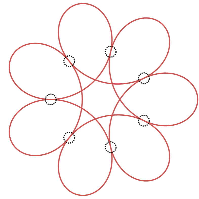
From Part 1 recall the spirograph function and its derivative:

$$\begin{array}{cc}s\left(\theta \right)& =p{e}^{-ib\theta }+b{e}^{i\theta }\\ \frac{ds}{d\theta }\left(\theta \right)& =-ibp{e}^{-ib\theta }+ib{e}^{i\theta }\end{array}$$

We want to constrain these equations to the points where the petals of the spirograph are tangent:

The critical thing to observe is that at the points of tangency, $\theta =\omega$, both the position and velocity vectors are parallel. This means that the tangent of their arguments (i.e. angle) are equal:

$$\begin{array}{cc}\tan \left(\arg \right(s\left(\omega \right)\left)\right)& =\tan \left(\arg \right(\frac{ds}{d\theta }\left(\omega \right)\left)\right)\\ \tan \left(\arctan \right(\frac{Im\left(s\right(\omega \left)\right)}{Re\left(s\right(\omega \left)\right)}\left)\right)& =\tan \left(\arctan \right(\frac{Im\left(\frac{ds}{d\theta }\right(\omega \left)\right)}{Re\left(\frac{ds}{d\theta }\right(\omega \left)\right)}\left)\right)\\ \frac{Im\left(s\right(\omega \left)\right)}{Re\left(s\right(\omega \left)\right)}& =\frac{Im\left(\frac{ds}{d\theta }\right(\omega \left)\right)}{Re\left(\frac{ds}{d\theta }\right(\omega \left)\right)}\\ Im\left(s\right(\omega \left)\right)\cdot Re\left(\frac{ds}{d\theta }\right(\omega \left)\right)& =Im\left(\frac{ds}{d\theta }\right(\omega \left)\right)\cdot Re\left(s\right(\omega \left)\right)& \text{(1)}\end{array}$$

For the sake of space, let's simplify each side separately. First the left side:

$$\begin{array}{c}Im\left(s\right(\omega \left)\right)\cdot Re\left(\frac{ds}{d\theta }\right(\omega \left)\right)\\ Im(p{e}^{-ib\omega }+b{e}^{i\omega })\cdot Re(-ibp{e}^{-ib\omega }+ib{e}^{i\omega })\\ \left(p\sin \right(-b\omega )+b\sin \omega )\cdot Re(-bp{e}^{i(\frac{\pi }{2}-b\omega )}+b{e}^{i(\frac{\pi }{2}+\omega )})\\ (-p\sin (b\omega )+b\sin \omega )\cdot (-bp\cos (\frac{\pi }{2}-b\omega )+b\cos (\frac{\pi }{2}+\omega \left)\right)\\ (-p\sin (b\omega )+b\sin \omega )\cdot (-bp\sin (b\omega )-b\sin \omega )\\ b{p}^2{\sin }^2\left(b\omega \right)+bp\sin \left(b\omega \right)\sin \omega -b^{2}p\sin \omega \sin \left(b\omega \right)-b^2{\sin }^2\omega \\ b{p}^2{\sin }^2\left(b\omega \right)+(1-b)bp\sin \left(b\omega \right)\sin \omega -b^2{\sin }^2\omega & \text{(2)}\end{array}$$

Now let's simplify the right side of $\text{(1)}$:

$$\begin{array}{c}Im\left(\frac{ds}{d\theta }\right(\omega \left)\right)\cdot Re\left(s\right(\omega \left)\right)\\ Im(-ibp{e}^{-ib\omega }+ib{e}^{i\omega })\cdot Re(p{e}^{-ib\omega }+b{e}^{i\omega })\\ Im(-bp{e}^{i(\frac{\pi }{2}-b\omega )}+b{e}^{i(\frac{i}{2}+\omega )})\cdot \left(p\cos \right(-b\omega )+b\cos \omega )\\ (-bp\sin (\frac{\pi }{2}-b\omega )+b\sin (\frac{\pi }{2}+\omega \left)\right)\cdot \left(p\cos \right(b\omega )+b\cos \omega )\\ (-bp\cos (b\omega )+b\cos \omega )\cdot \left(p\cos \right(b\omega )+b\cos \omega )\\ -b{p}^2{\cos }^2\left(b\omega \right)-b^{2}p\cos \left(b\omega \right)\cos \omega +bp\cos \omega \cos \left(b\omega \right)+b^2{\cos }^2\omega \\ -b{p}^2{\cos }^2\left(b\omega \right)+(1-b)bp\cos \left(b\omega \right)\cos \omega +b^2{\cos }^2\omega & \text{(3)}\end{array}$$

Now equate $\text{(3)}$ and $\text{(2)}$ per $\text{(1)}$. Group ${\sin }^2\omega +{\cos }^2\omega$ terms:

$$\begin{array}{cc}& b{p}^2{\sin }^2\left(b\omega \right)+(1-b)bp\sin \left(b\omega \right)\sin \omega -b^2{\sin }^2\omega =\\ & -b{p}^2{\cos }^2\left(b\omega \right)+(1-b)bp\cos \left(b\omega \right)\cos \omega +b^2{\cos }^2\omega \end{array}$$ $$\begin{array}{cc}& b{p}^2{\sin }^2\left(b\omega \right)+b{p}^2{\cos }^2\left(b\omega \right)-b^2{\sin }^2\omega -b^2{\cos }^2\omega =\\ & (1-b)bp\cos \left(b\omega \right)\cos \omega -(1-b)bp\sin \left(b\omega \right)\sin \omega \end{array}$$ $$b{p}^2-b^2=(1-b)bp\cdot \left(\cos \right(b\omega )\cos \omega -\sin (b\omega \left)\sin \omega \right)$$

Replace $\cos \left(b\omega \right)\cos \omega$ with $\cos \left(\right(b+1\left)\omega \right)+\sin \left(b\omega \right)\sin \omega$ per cosine angle sum formula:

$$\begin{array}{c}b\cdot (p^2-b)=(1-b)bp\cdot \left(\right(\cos \left(\right(b+1\left)\omega \right)+\sin \left(b\omega \right)\sin \omega )-\sin (b\omega \left)\sin \omega \right)\\ (p^2-b)=(1-b)p\cos \left(\right(b+1\left)\omega \right)\\ \frac{(p^2-b)}{(1-b)p}=\cos \left(\right(b+1\left)\omega \right)& \text{(4)}\end{array}$$

With $\text{(4)}$ we have an expression that puts $\omega$ in terms of $b$ and $p$. Since we are interested in solving for $p$ as $b\to \infty$, let's take the limit. Important to note that we assume $p$ exists as $b\to \infty$ during these steps:

$$\begin{array}{cc}\underset{b\to \infty }{lim}\cos \left(\right(b+1\left)\omega \right)& =\underset{b\to \infty }{lim}\frac{(p^2-b)}{(1-b)p}\\ \underset{b\to \infty }{lim}\cos \left(\right(b+1\left)\omega \right)& =\underset{b\to \infty }{lim}(\frac{p^2}{(1-b)p}-\frac{b}{(1-b)p})\\ \underset{b\to \infty }{lim}\cos \left(\right(b+1\left)\omega \right)& =\underset{b\to \infty }{lim}\frac{p}{(1-b)}+\underset{b\to \infty }{lim}\frac{b}{(b-1)p}\\ \underset{b\to \infty }{lim}\cos \left(\right(b+1\left)\omega \right)& =\frac{1}{p}\\ \underset{b\to \infty }{lim}(b+1)\omega & =\arccos \left(\frac{1}{p}\right)\\ \underset{b\to \infty }{lim}\omega & =\underset{b\to \infty }{lim}\frac{\arccos \left(\frac{1}{p}\right)}{b+1}& \text{(5)}\end{array}$$

Since we have assumed that $p$ exists as $b\to \infty$ it should be clear that ${lim}_{b\to \infty }\omega =0$ but we keep it in this form because it will be necessary to evaluate another limit.

The second major thing to observe is that at the points of tangency, $\frac{\pi n}{(b+1)}=\arg \left(s\right(\omega \left)\right)$, where $n\in Z$:

$$\begin{array}{cc}\frac{\pi n}{(b+1)}& =\arg \left(s\right(\omega \left)\right)\\ \frac{\pi n}{(b+1)}& =\arctan \left(\frac{Im\left(s\right(\omega \left)\right)}{Re\left(s\right(\omega \left)\right)}\right)\\ \tan \left(\frac{\pi n}{(b+1)}\right)& =\frac{Im\left(s\right(\omega \left)\right)}{Re\left(s\right(\omega \left)\right)}\\ \tan \left(\frac{\pi n}{(b+1)}\right)& =\frac{Im(p{e}^{-ib\omega }+b{e}^{i\omega })}{Re(p{e}^{-ib\omega }+b{e}^{i\omega })}\\ \tan \left(\frac{\pi n}{(b+1)}\right)& =\frac{p\sin (-b\omega )+b\sin \omega }{p\cos (-b\omega )+b\cos \omega }\\ \tan \left(\frac{\pi n}{(b+1)}\right)& =\frac{-p\sin \left(b\omega \right)+b\sin \omega }{p\cos \left(b\omega \right)+b\cos \omega }& \text{(6)}\end{array}$$

Now take the limit of $\text{(6)}$ as $b\to \infty$ and replace $\omega$ with $\text{(5)}$:

$$\begin{array}{cc}\underset{b\to \infty }{lim}\tan \left(\frac{\pi n}{(b+1)}\right)& =\underset{b\to \infty }{lim}\frac{-p\sin \left(b\frac{\arccos \left(\frac{1}{p}\right)}{b+1}\right)+b\sin (\frac{\arccos \left(\frac{1}{p}\right)}{b+1})}{p\cos \left(b\frac{\arccos \left(\frac{1}{p}\right)}{b+1}\right)+b\cos \left(\frac{\arccos \left(\frac{1}{p}\right)}{b+1}\right)}\\ \underset{b\to \infty }{lim}\tan \left(\frac{\pi n}{(b+1)}\right)& =\underset{b\to \infty }{lim}\frac{-p\sin \left(\arccos \left(\frac{1}{p}\right)\right)+b\sin \left(\frac{\arccos \left(\frac{1}{p}\right)}{b+1}\right)}{p\cos \left(\arccos \left(\frac{1}{p}\right)\right)+b\cos \left(\frac{\arccos \left(\frac{1}{p}\right)}{b+1}\right)}\end{array}$$

Use the identities $\cos \left(\arccos x\right)=x$ and $\sin \left(\arccos x\right)=\sqrt{1-x^2}$:

$$\begin{array}{cc}\underset{b\to \infty }{lim}\tan \left(\frac{\pi n}{(b+1)}\right)& =\underset{b\to \infty }{lim}\frac{-p\sqrt{1-(\frac{1}{p}{)}^2}+b\sin \left(\frac{\arccos \left(\frac{1}{p}\right)}{b+1}\right)}{p\left(\frac{1}{p}\right)+b\cos \left(\frac{\arccos \left(\frac{1}{p}\right)}{b+1}\right)}\\ \underset{b\to \infty }{lim}\tan \left(\frac{\pi n}{(b+1)}\right)& =\underset{b\to \infty }{lim}\frac{-\sqrt{p^2-1}+b\sin \left(\frac{\arccos \left(\frac{1}{p}\right)}{b+1}\right)}{1+b\cos \left(\frac{\arccos \left(\frac{1}{p}\right)}{b+1}\right)}\end{array}$$

Use the small-angle approximations for $\tan$, $\sin$, and $\cos$:

$$\begin{array}{cc}\underset{b\to \infty }{lim}\frac{\pi n}{(b+1)}& =\underset{b\to \infty }{lim}\frac{-\sqrt{p^2-1}+b\left(\frac{\arccos \left(\frac{1}{p}\right)}{b+1}\right)}{1+b}\\ \pi n& =-\sqrt{p^2-1}+\arccos \left(\frac{1}{p}\right)\\ \sqrt{p^2-1}& =\arccos \left(\frac{1}{p}\right)-\pi n\\ p^2-1& =\left(\arccos \right(\frac{1}{p})-\pi n{)}^2\\ p^2& =1+\left(\arccos \right(\frac{1}{p})-\pi n{)}^2& \text{(7)}\end{array}$$

If we set $n=-1$ then $\text{(7)}$ is exactly equal to the equation characterizing entry A328227 in the OEIS. Important to note that only the negative solutions of $p$ when $n>0$ are valid and only the positive solutions of $p$ when $n\le 0$ are valid.

As we mentioned in the previous article, different values of $n$ result in different solutions for $p$. This is because the tangency condition is satisfied by multiple shapes of the spirograph. The number of distinct values of $p$ that result in unique shapes is $\lfloor b/2\rfloor$ and when $b\to \infty$, there are an infinite number of values for $p$. To capture the fact that this is a family of numbers, we'll rename $p$ to $P{P}_n^b$ and rephrase $\text{(7)}$ given the domain considerations in the previous paragraph. $P{P}_n^{\infty }$ are the positive solutions of the following equation, for $n\in Z^{\ast }$:

$$\begin{array}{}(P{P}_n^{\infty }{)}^2& =1+\left(\arccos \right(\frac{1}{P{P}_n^{\infty }})+\pi n{)}^2& \text{(8)}\end{array}$$

Proof That $P{P}_{n\ne 0}^{\infty }$ is Transcendental

Our original proof that $P{P}_{n\ne 0}^{\infty }$ is transcendental had an incorrect step. Reddit user existentialpenguin suggested a variation on the original proof which the following proof incorporates. This proof relies on the Lindemann–Weierstrass theorem which for our purposes implies that if $x$ is a algebraic number then $\cos x$ must be a transcendental number or $x=0$. Before engaging in the main proof, we first want to show that when $P{P}_n^{\infty }=1$ then $n=0$:

$$\begin{array}{c}(P{P}_n^{\infty }{)}^2=1+(\arccos \left(\frac{1}{P{P}_n^{\infty }}\right)+\pi n{)}^2\\ 1^2=1+\left(\arccos \right(\frac{1}{1})+\pi n{)}^2\\ 1=1+\left(\arccos \right(1)+\pi n{)}^2\\ 0=\pi n\\ 0=n& \text{(9)}\end{array}$$

Now for the main proof, we'll put $\text{(8)}$ into a more convenient form:

$$\begin{array}{c}(P{P}_{n\ne 0}^{\infty }{)}^2=1+(\arccos \left(\frac{1}{P{P}_{n\ne 0}^{\infty }}\right)+\pi n{)}^2\\ +\sqrt{(P{P}_{n\ne 0}^{\infty }{)}^2-1}=\arccos \left(\frac{1}{P{P}_{n\ne 0}^{\infty }}\right)+\pi n\\ \cos (+\sqrt{(P{P}_{n\ne 0}^{\infty }{)}^2-1})=\cos \left(\arccos \right(\frac{1}{P{P}_{n\ne 0}^{\infty }})+\pi n)\\ \cos (+\sqrt{(P{P}_{n\ne 0}^{\infty }{)}^2-1})=\left(\frac{1}{P{P}_{n\ne 0}^{\infty }}\right)\cos \left(\pi n\right)-\left(\frac{1}{P{P}_{n\ne 0}^{\infty }}\right)\sin \left(\pi n\right)\\ (-1{)}^n\cos (+\sqrt{(P{P}_{n\ne 0}^{\infty }{)}^2-1})=(\frac{1}{P{P}_{n\ne 0}^{\infty }})\\ \frac{(-1{)}^n}{\cos (+\sqrt{(P{P}_{n\ne 0}^{\infty }{)}^2-1})}=P{P}_{n\ne 0}^{\infty }& \text{(10)}\end{array}$$

$\text{(9)}$ shows that when $P{P}_n^{\infty }=1$ then it is implied that $n=0$. By the contrapositive that means that when $n\ne 0$ then $P{P}_n^{\infty }\ne 1$. Now let's use $\text{(10)}$ and proceed by contradiction:

• Assume that $P{P}_{n\ne 0}^{\infty }\ne 1$ is algebraic.
• Then $(P{P}_{n\ne 0}^{\infty }{)}^2$ must be algebraic.
• Then $(P{P}_{n\ne 0}^{\infty }{)}^2-1$ must be algebraic.
• Then $(P{P}_{n\ne 0}^{\infty }{)}^2-1$ must be algebraic.
• Then $+\sqrt{(P{P}_{n\ne 0}^{\infty }{)}^2-1}$ must be algebraic.
• Then $\cos (+\sqrt{(P{P}_{n\ne 0}^{\infty }{)}^2-1})$ must be transcendental.
• Then $\frac{(-1{)}^n}{\cos (+\sqrt{(P{P}_{n\ne 0}^{\infty }{)}^2-1})}$ must be transcendental.
• Yet, $P{P}_{n\ne 0}^{\infty }=\frac{(-1{)}^n}{\cos (+\sqrt{(P{P}_{n\ne 0}^{\infty }{)}^2-1})}$ which we assumed was algebraic, a contradiction.

Therefore $P{P}_{n\ne 0}^{\infty }$ must be transcendental. $\square$

Computing $P{P}_n^{\infty }$

Given our equation for $P{P}_n^{\infty }$ there is no algebraically straightforward way to compute $P{P}_n^{\infty }$. Though maybe with a simple change of variables we can simplify the problem. Let's set $P{P}_n^{\infty }=\frac{1}{\cos (q_n-\pi n)}$:

$$\begin{array}{cc}(P{P}_n^{\infty }{)}^2& =1+\left(\arccos \right(\frac{1}{P{P}_n^{\infty }})+\pi n{)}^2\\ (\frac{1}{\cos (q_n-\pi n)}{)}^2& =1+\left(\arccos \right(\frac{1}{\frac{1}{\cos (q_n-\pi n)}})+\pi n{)}^2\\ \frac{1}{{\cos }^2(q_n-\pi n)}& =1+\left(\arccos \right(\cos (q_n-\pi n))+\pi n{)}^2\\ \frac{1}{{\cos }^2(q_n-\pi n)}& =1+q_n^2& {\cos }^2(q_n-\pi n)& =\frac{1}{1+q_n^2}\\ \cos (q_n-\pi n)& =\frac{1}{\pm \sqrt{1+q_n^2}}\\ \text{(11)}\end{array}$$

Now let's replace $\cos (q_n-\pi n)$ using the identity $\cos (q_n-\pi n)=\frac{1}{\pm \sqrt{1+{\tan }^2(q-\pi n)}}$:

$$\begin{array}{cc}\frac{1}{\pm \sqrt{1+{\tan }^2(q_n-\pi n)}}& =\frac{1}{\pm \sqrt{1+q_n^2}}\\ \tan (q_n-\pi n)& =q_n\\ \tan q_n& =q_n\\ \tan q_n-q_n& =0\end{array}$$

We have reduced our original problem to the problem of finding the roots of $\tan x-x$, i.e. the fixed points of $\tan x$. The specific root we need for $P{P}_n^{\infty }$ is the smallest root $\ge \pi n$, which we call $q_n$, because otherwise $\arccos \left(\cos \right(x-\pi n\left)\right)\ne x-\pi n$. The fixed points of $\tan x$ are well-known numbers in themselves that have applications in many areas of math, science, and engineering. There are a few known methods for computing them already (you'll find one in the addendum to this article). You can find more info at MathWorld, including the first 6 roots. For our purposes it suffices to show the connections between the $n$th fixed point of $\tan x$ and $P{P}_n^{\infty }$.

The first connection is from our original change of variables:

$$\begin{array}{cc}P{P}_n^{\infty }& =\frac{1}{\cos (q_n-\pi n)}& P{P}_n^{\infty }& =\frac{1}{\cos q_n\cos \left(\pi n\right)+\sin q_n\sin \left(\pi n\right)}\\ P{P}_n^{\infty }& =\frac{1}{(-1{)}^n\cos q_n}\\ P{P}_n^{\infty }& =(-1{)}^n\sec q_n\\ \text{(12)}\end{array}$$

We can derive the other connection by combining $\text{(11)}$ and $\text{(12)}$:

$$\begin{array}{cc}\frac{1}{{\cos }^2(q_n-\pi n)}& =1+q_n^2\\ (P{P}_n^{\infty }{)}^2& =1+q_n^2\\ P{P}_n^{\infty }& =+\sqrt{1+q_n^2}\end{array}$$

The two different methods of converting between the fixed points of $\tan x$ and $P{P}_n^{\infty }$ is incredible and is a direct result of $q_n$'s nature as both an argument and a result of $\tan x$.

Conclusion

So what is $P{P}_n^{\infty }$? On a physical and geometrical basis, we can say that it's the secant of the right triangle whose tangent is equivalent in radians to the angle to which these ratios are relative. $P{P}_n^{\infty }$ and the fixed points of $\tan x$ are the shadows of these special triangles, of which there are an infinite amount. I have to imagine that the angles and ratios which characterize these special triangles show up in various problems. The spirograph just happened to be my window to them. $P{P}_1^{\infty }$ shows up as the solution to this IBM challenge problem, about which Numberphile also made a video. May there be other problems where the other ratios of this special triangle are relevant, i.e. the sine, cosine, cosecant, or cotangent?

Given that $P{P}_n^{\infty }$ have a well-understood connection to the fixed points of $\tan x$, I now think that the values of $P{P}_n^b$ which correspond to finite values of $b$ that we derived in Part 1 are more enigmatic and interesting. In a way they could be understood as "intermediate solutions" toward the fixed points of $\tan x$. I find this fascinating and in a future article I may derive a series expansion for directly computing those intermediate solutions. They may reveal more structure and properties of the fixed points of $\tan x$.

Rian Hunter, 6/16/21

Addendum: Computing the Fixed Points of $\tan x$

To compute the roots of $\tan x-x$, we can apply its series reversion, $f\left(x\right)$, to $0$ to solve for $x$. Unfortunately for the series reversion algorithm to work, we need the first-order term to be non-zero. The series expansion of $\tan x$ is $x+\frac{x^3}{3}+\frac{2x^5}{15}+\dots$, so the expansion of $\tan x-x$ is $\frac{x^3}{3}+\frac{2x^5}{15}+\dots$ which is no good. To fix this, make a change of variables that takes advantage of the fact that $\tan (\frac{\pi }{2}-x)=\cot x$ and $\cot (x+\pi n)=\cot x$, i.e. $q_n=\pi n+\frac{\pi }{2}-r$, where $n\in Z^{\ast }$ results in a solution for the $n$th fixed point of $\tan x$:

$$\begin{array}{cc}\tan q_n-q_n& =0\\ \tan (\pi n+\frac{\pi }{2}-r)-(\pi n+\frac{\pi }{2}-r)& =0\\ \tan (\frac{\pi }{2}-(r-\pi n\left)\right)+r& =\pi n+\frac{\pi }{2}\\ \cot (r-\pi n)+r& =\pi n+\frac{\pi }{2}\\ \cot \left(r\right)+r& =\pi n+\frac{\pi }{2}\end{array}$$

Yet there is another snag. Ideally we would use the Taylor series of $\cot r+r$ about $r=0$ to derive the forward series coefficients but $\cot r+r$ is not defined at $r=0$. On the other hand $\frac{1}{\cot r+r}$ is, so we'll use that instead:

$$\begin{array}{}\frac{1}{\cot \left(r\right)+r}& =\frac{1}{\pi n+\frac{\pi }{2}}& \text{(13)}\end{array}$$

At this stage the next step would be to find the derivatives of $g\left(x\right)=\frac{1}{\cot \left(r\right)+r}$ to get a formula for the series coefficients parameterized by a series index, e.g. $k$, but unfortunately there is no easily discernable pattern of the value of the derivatives of $\frac{1}{\cot x+x}$ at $x=0$. The series reversion algorithm is also not very amenable to a compact notation. A Python script to compute the series reversion coefficients will be provided at the end of this section. Additionally the OEIS provides the numerators and the denominators. For the sake of simplicity we'll assume we have the series reversion coefficients readily available as $d_k$ and we'll define the reversion polynomial as $f\left(x\right)$:

$$\begin{array}{c}f\left(x\right)=\sum _{k=0}^{\infty }{d}_k{x}^k\end{array}$$

We can then apply $f\left(x\right)$ to $\text{(13)}$:

$$\begin{array}{cc}f\left(\frac{1}{\cot r+r}\right)& =f\left(\frac{1}{\pi n+\frac{\pi }{2}}\right)\\ r& =f\left(\frac{1}{\pi n+\frac{\pi }{2}}\right)\\ \pi n+\frac{\pi }{2}-q_n& =f\left(\frac{1}{\pi n+\frac{\pi }{2}}\right)\\ q_n& =\pi n+\frac{\pi }{2}-f\left(\frac{1}{\pi n+\frac{\pi }{2}}\right)\\ q_n& =\pi n+\frac{\pi }{2}-\sum _{k=0}^{\infty }{d}_k\cdot (\frac{1}{\pi n+\frac{\pi }{2}}{)}^k\end{array}$$

Now back to the detail of computing $d_k$, the following Python script shows how to compute $d_k$ and using them to compute $q_n$:

import sympy as sp

import sys

try:
    num_terms = int(sys.argv[1])
except IndexError:
    num_terms = 10

try:
    num_fixed_points = int(sys.argv[2])
except IndexError:
    num_fixed_points = 10

x = sp.symbols('x', real=True)
y = 1 / (sp.cot(x) + x)
s = sp.series(y, x, 0, num_terms)

# this is necessary for the series reversion
# algorithm to work
assert not s.coeff(x, 0)
assert s.coeff(x, 1)

s = s.removeO()

y2 = sp.symbols('y', real=True)
coeffs = sp.symbols('a1:' + str(num_terms), real=True)
finv = sum(sym * y2 ** (i + 1) for (i, sym) in enumerate(coeffs))

newy = s.subs(x, finv).expand()

eqs = []
for i in range(0, num_terms - 1):
    val = newy.coeff(y2 ** (i+1))

    if not i:
        expected = 1
    else:
        expected = 0

    eqs.append(sp.Eq(val, expected))

sols = sp.solve(eqs)
if isinstance(sols, list):
    sols = sols[0]

print("Here are the first %d coefficients for the series reversion of 1/(cot(x) + x)" % (num_terms,))
print(0, 0)
for (k, sym) in enumerate(coeffs):
    print(k+1, sols[sym])

print()

finv_real = sum(sols[sym] * y2 ** (i + 1) for (i, sym) in enumerate(coeffs))
print("Here are approximations for the first %d fixed points of tan(x)" % (num_fixed_points,))
for k in range(num_fixed_points):
    q = (2 * k + 1) * sp.pi/2
    print(k, (q - finv_real.subs(y2, 1/q)).evalf())